Personalized metabolic power

OmniBandBridge’s power number is metabolic power: the rate at which your body burns energy while you walk or run, in watts. It is not the mechanical, Stryd-style wattage — it’s the physiological cost of the effort, and OBB calibrates it on you, workout after workout. This page explains the model end to end.

Runner or walker — it works for both

Metabolic power is gait-agnostic: it’s energy per unit time, defined the same way whether you run or walk. That’s a real difference from mechanical running power (Stryd-style), which is a running-biomechanics construct that doesn’t translate to walking. So OBB’s core metric is the right one for brisk / incline walking too — an audience that’s larger than runners, and one where training by incline and heart rate (rather than high-intensity intervals) is exactly what’s often recommended. Everything below applies to walkers as much as runners.

Step 1 — The baseline: Minetti’s cost of transport

The starting point is the most-cited model in the literature for walking/running on gradients, Minetti et al. (2002) (Journal of Experimental Biology) — which publishes cost-of-transport curves for both walking and running. It gives the energy cost per kg per metre as a function of the grade i (decimal — flat = 0, 5% uphill = 0.05, downhill negative):

Running:  Cmet(i) = 155.4·i⁵ − 30.4·i⁴ − 43.3·i³ + 46.3·i² + 19.5·i + 3.6   [J/(kg·m)]
Walking:  Cmet(i) = 280.5·i⁵ − 58.7·i⁴ − 76.8·i³ + 51.9·i² + 19.6·i + 2.5   [J/(kg·m)]

Multiply by speed and body mass and you get power:

P [W]    = Cmet(i, gait) × v [m/s] × mass [kg]
P [W/kg] = Cmet(i, gait) × v            ← comparable across people

The two inputs, speed and grade, are exactly what OBB already collects: on a treadmill from FTMS or manual entry (the ideal case — both values are exact), outdoors from GPS + DEM elevation maps.

Why grade matters so much

The polynomial is steep: at the same speed, a 6% incline roughly doubles the energy cost of flat locomotion. That’s why OBB invests so much in getting the grade right (FTMS indoors, offline DEM maps outdoors).

Step 1b — Walking vs running: the right curve, automatically

The two curves are genuinely different — walking is cheaper on the flat (baseline 2.5 vs 3.6) and scales differently with the grade — so using the running curve for a walker (or vice-versa) mis-costs the effort. OBB picks the correct curve per sample, not once for the whole workout, so a session that mixes a walking warm-up, a run, and a walking cool-down is costed correctly throughout.

How the gait is decided, in order:

• Aerial phase. A running foot leaves the ground; a walking one never does. If the footpod reports flight time or vertical oscillation, it’s running — but only above walking speed, because the Mi Band can report a spurious flight time during brisk incline walking (validated on real data: without this guard, 4–5 km/h walks were wrongly flagged as running).
• Speed otherwise (for sensors without footpod dynamics, or footpod walking): a walk↔run threshold with hysteresis so it doesn’t flip-flop at the transition.

Walking also depends on speed

Running’s cost per metre is roughly independent of speed, but walking’s is U-shaped: there’s an optimal walking speed (~4.7 km/h) and going slower or faster costs more per metre. OBB corrects for this with a one-parameter factor that is 1 at the optimum and grows as you move away from it:

φ(v) = ½·(v_opt/v + v/v_opt)      applied to the walking curve only

So a slow 3 km/h walk is costed a few percent higher per metre than a brisk one — small near the optimum, larger at the extremes. (Metabolic power still stays finite even at very low speed.)

Why this matters for walkers

These refinements make the absolute metabolic power — and therefore your calories and your personal thresholds — physiologically right for walking, not just running. It’s what lets OBB serve incline walkers as a first-class use case, not an afterthought.

Step 2 — Why personalize it

Minetti is a population average. Two runners at the same speed and grade get the same number, regardless of fitness, body composition or running form. OBB’s distinctive move is to fit the model to you — using the one physiological signal every runner can measure: heart rate.

The key idea: at a steady effort, your steady-state HR is a proxy for your metabolic cost. If OBB knows how your HR responds to a given metabolic power, it holds a personal calibration curve — and everything downstream (zones, thresholds, day-form) becomes personal too.

Step 3 — Collecting calibration points

Every workout is a potential calibration session. After each activity, OBB scans the recording for steady-state plateaus: stretches where speed and grade are constant and the HR has stabilised (the first minutes after each change are discarded — HR needs 2–3 minutes to settle, so only the final part of each plateau is used).

Each plateau becomes one calibration point: (P_Minetti, average HR) — stored in the local database, together with the biomechanical averages (ground contact time, cadence, vertical ratio, impact) that feed the Phase-2 personal correction (Step 6). A dedicated calibration session (e.g. 5–6 min blocks stepping the incline at constant speed) fills the grid faster, but it’s optional: normal training accumulates points on its own.

Because fitness changes over time, the fit uses a rolling time window (~60–90 days), so the curve tracks your current shape, not last year’s.

Step 4 — The fit

With enough points, OBB fits the personal HR–power relationship with two candidate models:

HR = a·P + c        (linear)
HR = a·P^b          (power law — the standard in the literature)

Both are fitted by ordinary least squares in closed form (the power law in log space: ln HR = ln a + b·ln P) — no heavy libraries, fully on-device.

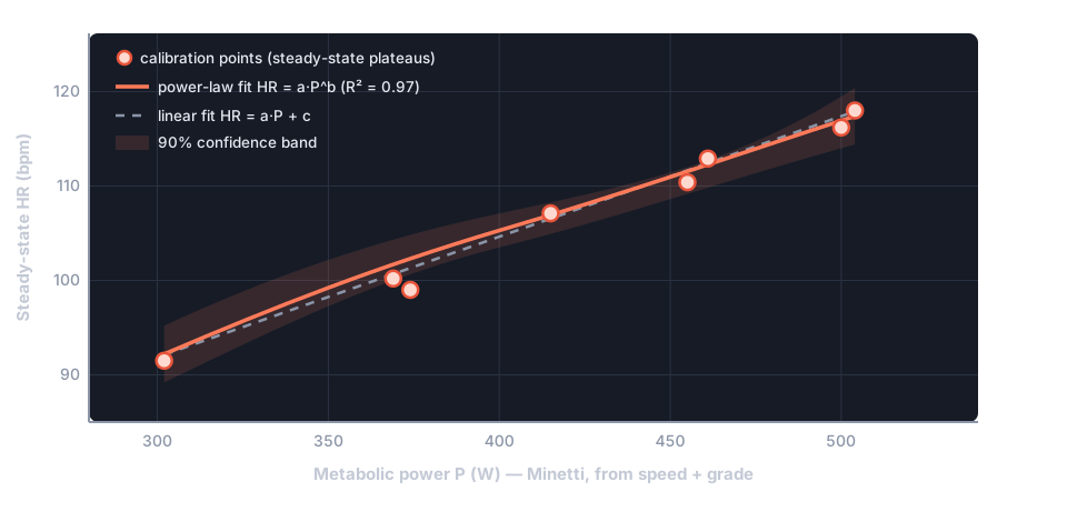
The chart above is what OBB’s Personal Power Profile screen shows:

• Points — your steady-state plateaus, P on the x-axis, average HR on the y-axis.
• Curves — the fitted models, drawn only across the calibrated range (extrapolating a regression outside its data would be misleading — a straight line would happily predict an absurd HR at P = 0).
• Confidence band — the shaded region is the 90% confidence interval for the mean response, computed in closed form from the residual variance (Student’s t). It’s narrowest in the middle of your data and flares at the edges — a visual honesty indicator.

How good is the fit? R² and RMSE

• R² measures the fraction of HR variability explained by power (R² = 1 − SS_res/SS_tot). An R² of 0.9+ means the curve tracks your points closely — but with few points R² is optimistic, so OBB also reports the RMSE in bpm (“the model is off by ±X beats on average”), which is easier to judge.
• Linear vs power law: over a narrow power range the two are nearly indistinguishable (any monotone curve looks like a line). Over a wider range the power law usually wins, because HR physiologically saturates toward its maximum.
• Every coefficient comes with a 90% confidence interval (t-distribution, asymmetric for the power-law a since it’s exponentiated back from log space), shown as error bars in the profile screen.

Step 5 — What the curve is for: inversion

The fit gives HR = f(P); the practical value is mostly in the inverse, P = f⁻¹(HR):

Model	Direct (P → HR)	Inverse (HR → P)
Linear	HR = a·P + c	P = (HR − c) / a
Power law	HR = a·P^b	P = (HR / a)^(1/b)

• Personal power zones. Your HR zone boundaries become boundaries in watts — so you can train by power, which reacts instantly to speed/grade changes, instead of HR, which lags by 30–60 seconds. The Stryd principle — but calibrated on your physiology.
• Day-form indicator. At a given power the model predicts your expected HR; if today’s measured HR is consistently higher at the same power, you’re fatigued (or hot, or dehydrated) — an objective freshness check.
• Session planning. “I want to stay in Z2” → the model returns the watt range, and since P depends on speed and grade, the treadmill combinations that land there.

Terms like “FTP” and “zones” for walkers

These names come from running and cycling, but the idea carries over: your “threshold” is simply the sustainable metabolic effort that’s personal to you, and the zones are bands of that effort — equally meaningful for incline walking. OBB reuses the familiar terms rather than inventing new ones; read them as sustainable effort and effort zones if you train by walking.

Step 6 — Biomechanics in the loop (Phase 2)

The Phase-1 fit uses speed and grade only, so at fixed v/grade the power is constant. Phase 2 folds in the advanced running-dynamics metrics (ground contact time, cadence, impact, vertical ratio — see Supported devices) as a personal, multiplicative correction on the cost:

P_corretta = P_Minetti · f ,   f = 1 + Σ γ_j · z_j     (z = standardised feature)
HR = a · (P_Minetti · f)^b

Standardising each feature (z-score) makes the weights γ_j comparable regardless of units. And there’s a neat trick: taking logs turns the whole thing into an ordinary least-squares regression of ln HR on [ln P, z_GCT, z_cad, z_imp, z_VSR] — still closed-form, on-device, no heavy solver. Phase 1 (the plain power law) is exactly the nested reduced model [ln P], so the two are compared honestly on the same points with adjusted R², RMSE and leave-one-out cross-validation.

It switches itself on only when it earns it. OBB adopts the correction only if Phase 2 generalises better than Phase 1 under cross-validation; otherwise it gracefully stays on plain Minetti (f ≈ 1). The upgrade can’t make the estimate worse.

Source-agnostic: it uses whatever your device measures

The fit is source-agnostic. Each metric becomes a regressor only if your device actually provides it (and it varies across your points); anything missing is simply dropped, without discarding those points. So the model adapts to a Mi Band, a UA Atlas footpod, or a Garmin watch alike:

Regressor	Mi Band (footpod)	UA Atlas	Garmin (Connect IQ)
Ground contact time	✅	✅	✅
Cadence	✅	✅	✅
Vertical ratio	✅	—	✅
Impact	✅	—	—

Ground contact time is the universal backbone (every source measures it, and it carries genuine running-economy information independent of speed). Notably stride length is not a regressor: it’s almost fully determined by speed and cadence (stride ≈ 2·v/cadence), so it adds no independent information and would only introduce collinearity.

A live, personal instantaneous power

Once active, the correction is applied to the live metabolic power too — not just to the after-the-fact analysis. So at a fixed treadmill speed and incline your MEP is no longer flat: it breathes with your biomechanics — if fatigue lengthens your ground contact or your form drifts, the estimated cost rises even though speed and grade haven’t changed. The factor is clamped to a safe band so per-second values stay physiologically sane.

Honest by construction

If biomechanics don’t add explanatory power for you, cross-validation keeps Phase 1 and the model stays Minetti. It only ever adopts the extra terms when they demonstrably predict your heart rate better.